Advanced tutorials
Online Clustering of Temporal Activity (OCTA)
The OCTA network is a Buildingblock which implements a model
of the canonical microcircuit [1]. The canonical microcircuit, which itself is
an abstraction and generalisation of anatomical reality, is
found throughout cortical domains, i.e. visual, auditory, motor etc., and
throughout the hierarchy, i.e. primary sensory and pre-frontal cortex.
The objective of the OCTA BuildingBlock is to leverage the temporal
information of so-called event-based sensory systems which are completely
time-continuous [2]. The temporal information, or the precise timing
information of events, is used to extract spatio-temporal correlated
patterns from incoming streams of events. But also to learn temporally
structured, i.e ordered, sequences of patterns in order to perform temporal
predictions of future inputs.
A single OCTA BuildingBlock consists of two two-dimensional WTA
networks (compression and prediction) connected in a recurrent manner to a
relay (projection) population.
It is inspired by the connectivity between the different layers of the mammalian cortex: every element in the teili implementation has a cortical counterpart for which the connectivity and function is preserved:
compression[‘n_proj’] : Layer 4
compression[‘n_exc’] : Layer 2/3
prediction[‘n_exc’] : Layer 5/6
Given a high dimensional input in L2/3, the network extracts in the recurrent connections of L4 a lower dimensional representation of temporal dependencies by learning spatio-temporal features.
As in the other tutorials we start with importing the relevant libraries
import sys
import numpy as np

from pyqtgraph.Qt import QtGui
import pyqtgraph as pg
from brian2 import us, ms, prefs, defaultclock, core, float64
import copy as cp

from teili import TeiliNetwork
from teili.building_blocks.octa import Octa
from teili.models.parameters.octa_params import wta_params, octa_params,\
    mismatch_neuron_param, mismatch_synap_param
from teili.models.neuron_models import OCTA_Neuron as octa_neuron
from teili.stimuli.testbench import OCTA_Testbench
from teili.tools.sorting import SortMatrix
from teili.tools.visualizer.DataViewers import PlotSettings
from teili.tools.visualizer.DataControllers.Rasterplot import Rasterplot
from teili.tools.io import monitor_init
Now we set the code-generation target as well as the simulation time step.
Please note the small dt. In order to avoid integration errors and make sure that
the timing of spikes/events can be used we need to lower the simulation time step much more
than in our other (simpler) tutorials.
Note
The OCTA building block can not be run in standalone mode as it requires quite complicated run_regularly functions which are currently not available in c++.
prefs.codegen.target = "numpy"
defaultclock.dt = 0.1 * ms
core.default_float_dtype = float64
Now we can create the TeiliNetwork and load the specifically designed OCTA_Testbench.
# create the network
Net = TeiliNetwork()
OCTA_net = Octa(name='OCTA_net')

#Input into the Layer 4 block: compression['n_proj']
testbench_stim = OCTA_Testbench()
testbench_stim.rotating_bar(length=10, nrows=10,
                            direction='cw',
                            ts_offset=3, angle_step=10,
                            noise_probability=0.2,
                            repetitions=300,
                            debug=False)

OCTA_net.groups['spike_gen'].set_spikes(indices=testbench_stim.indices,
                                        times=testbench_stim.times * ms)
As in the other tutorials we can now add the different BuildingBlocks and sub_blocks to the network.
In order to visualise the input we need to explicitely add the monitor again, as we changed the
Neurons it is monitoring.
Net.add(OCTA_net,
        OCTA_net.monitors['spikemon_proj'],
        OCTA_net.sub_blocks['compression'],
        OCTA_net.sub_blocks['prediction'])

Net.run(np.max(testbench_stim.times) * ms,
        report='text')
The simulation will take about 10 minutes. In contrast to other tutorials we only provide a pyqtgraph backend visualisation, as the amount of data is too high and the way we want to look at the spiking activity needs a more sophisticated sub plot arrangement.
app = QtGui.QApplication.instance()
if app is None:
    app = QtGui.QApplication(sys.argv)
else:
    print('QApplication instance already exists: %s' % str(app))

pg.setConfigOptions(antialias=True)
labelStyle = {'color': '#FFF', 'font-size': 18}
MyPlotSettings = PlotSettings(fontsize_title=18,
                                fontsize_legend=12,
                                fontsize_axis_labels=14,
                                marker_size=10)
sort_rasterplot = True
win = pg.GraphicsWindow(title="Network activity")
win.resize(1024, 768)
p1 = win.addPlot(title="Spike raster plot: L4")
p2 = win.addPlot(title="Zoomed in spike raster plot: L2/3")
win.nextRow()
p3 = win.addPlot(title="Zoomed in spike raster plot: L5/6",
                    colspan=2)

p1.showGrid(x=True, y=True)
p2.showGrid(x=True, y=True)
p3.showGrid(x=True, y=True)

region = pg.LinearRegionItem()
region.setZValue(10)

p1.addItem(region, ignoreBounds=True)


monitor_p1 = OCTA_net.monitors['spikemon_proj']
monitor_p2 = monitor_init()
monitor_p2.i = cp.deepcopy(np.asarray(
    OCTA_net.sub_blocks['compression'].monitors['spikemon_exc'].i))
monitor_p2.t = cp.deepcopy(np.asarray(
    OCTA_net.sub_blocks['compression'].monitors['spikemon_exc'].t))
monitor_p3 = monitor_init()
monitor_p3.i = cp.deepcopy(np.asarray(
    OCTA_net.sub_blocks['prediction'].monitors['spikemon_exc'].i))
monitor_p3.t = cp.deepcopy(np.asarray(
    OCTA_net.sub_blocks['prediction'].monitors['spikemon_exc'].t))

if sort_rasterplot:
    weights_23 = cp.deepcopy(np.asarray(
        OCTA_net.sub_blocks['compression'].groups['s_exc_exc'].w_plast))
    s_23 = SortMatrix(nrows=OCTA_net.sub_blocks['compression'].groups['s_exc_exc'].source.N,
                        ncols=OCTA_net.sub_blocks['compression'].groups['s_exc_exc'].target.N,
                        matrix=weights_23,
                        axis=1)

    weights_23_56 = cp.deepcopy(np.asarray(
        OCTA_net.sub_blocks['prediction'].groups['s_inp_exc'].w_plast))
    s_23_56 = SortMatrix(nrows=OCTA_net.sub_blocks['prediction'].groups['s_inp_exc'].source.N,
                            ncols=OCTA_net.sub_blocks['prediction'].groups['s_inp_exc'].target.N,
                            matrix=weights_23_56,
                            axis=1)

    monitor_p2.i = np.asarray([np.where(
        np.asarray(s_23.permutation) == int(i))[0][0] for i in monitor_p2.i])
    monitor_p3.i = np.asarray([np.where(
        np.asarray(s_23_56.permutation) == int(i))[0][0] for i in monitor_p3.i])


duration = np.max(testbench_stim.times)
Rasterplot(MyEventsModels=[monitor_p1],
            MyPlotSettings=MyPlotSettings,
            time_range=[0, duration],
            neuron_id_range=None,
            title="Input rotating bar",
            xlabel='Time (s)',
            ylabel="Neuron ID",
            backend='pyqtgraph',
            mainfig=win,
            subfig_rasterplot=p1,
            QtApp=app,
            show_immediately=False)

Rasterplot(MyEventsModels=[monitor_p2],
            MyPlotSettings=MyPlotSettings,
            time_range=[0, duration],
            neuron_id_range=None,
            title="Spike raster plot of L2/3",
            xlabel='Time (s)',
            ylabel="Neuron ID",
            backend='pyqtgraph',
            mainfig=win,
            subfig_rasterplot=p2,
            QtApp=app,
            show_immediately=False)

Rasterplot(MyEventsModels=[monitor_p3],
            MyPlotSettings=MyPlotSettings,
            time_range=[0, duration],
            neuron_id_range=None,
            title="Spike raster plot of L5/6",
            xlabel='Time (s)',
            ylabel="Neuron ID",
            backend='pyqtgraph',
            mainfig=win,
            subfig_rasterplot=p3,
            QtApp=app,
            show_immediately=False)

region.sigRegionChanged.connect(update)
p2.sigRangeChanged.connect(updateRegion)
p3.sigRangeChanged.connect(updateRegion)
region.setRegion([29.6, 30])
p1.setXRange(25, 30, padding=0)

app.exec_()
The generated plot should look like this:
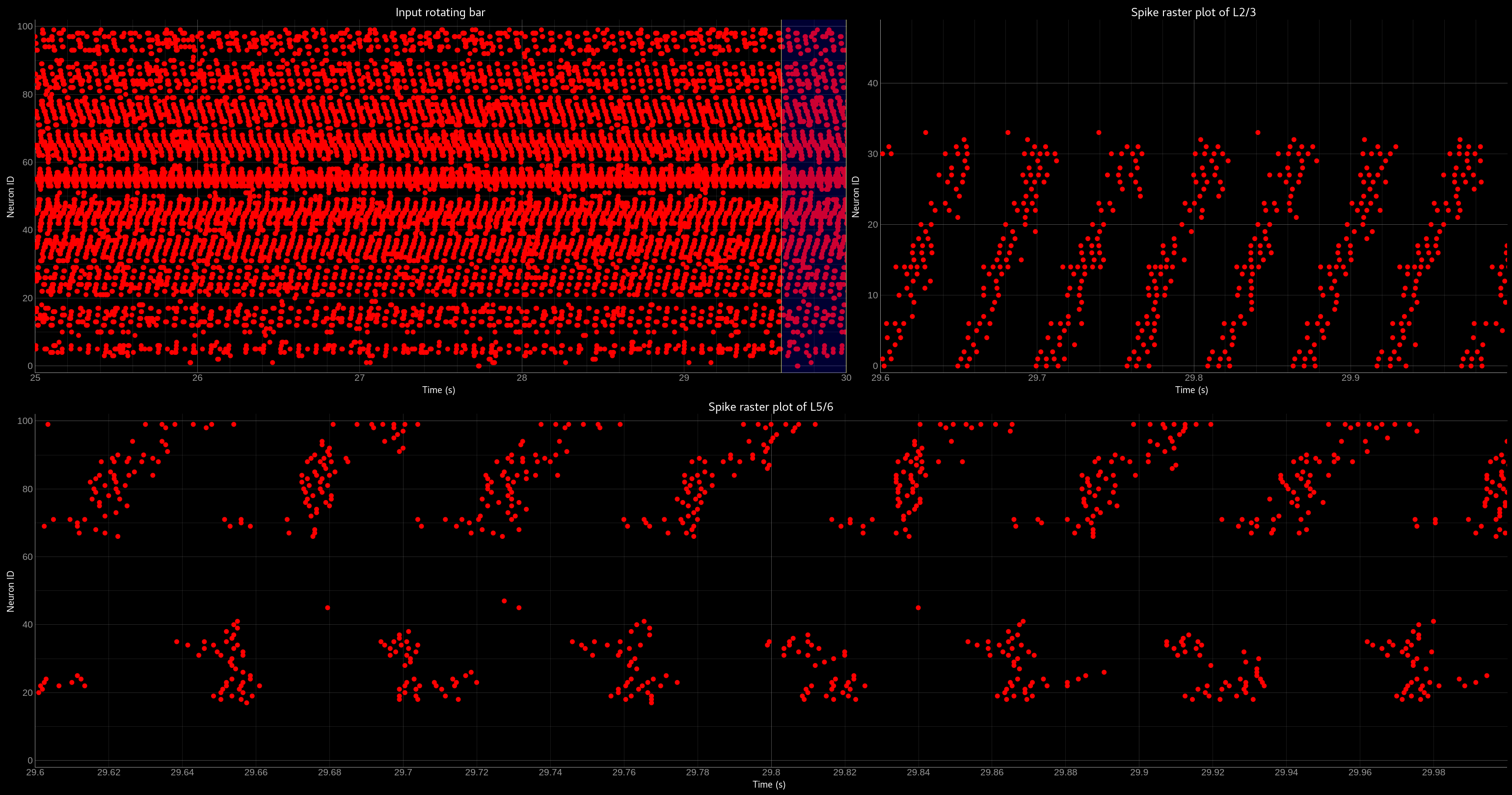
Network activity of the OCTA BuildingBlock.
Spike raster plot of the relay layer (L4, top left), the compression layer (L2/3, top right) and the prediction layer (L5/6, bottom).
The blue bar indicates the zoomed-in region of the spike raster plot of L2/3 and L5/6. Note that the spike raster plots are sorted
according to the recurrent weight matrix of L2/3 for the L2/3 spike raster plot and according to the L2/3 to L5/6 weights in the case
of the L5/6 spike raster plot. This sorting enables us to see the learned structure of the synaptic weights. In case of L2/3 we can see
that the temporally structured sequence is encoded in the recurrent weight matrix. In the case of L5/6 we can see that we can preserver
temporal information in recurrent connections, which then can be used to predict the input. For more information please refer to Milde 2019.
Three-way networks
The Threeway block is a BuildingBlock that implements a network of
three one-dimensional WTA populations A, B and C, connected to a hidden two-dimensional WTA population H.
The role of the hidden population is to encode a relation between A, B and C, which serve as inputs andor outputs.
In this example A, B and C encode one-dimensional values in range from 0 to 1 in a relation A + B = C to each other, which is hardcoded into connectivity of the hidden population.
To use the block instantiate it and add to the TeiliNetwork
from brian2 import ms, prefs, defaultclock

from teili.building_blocks.threeway import Threeway
from teili.tools.three_way_kernels import A_plus_B_equals_C
from teili import TeiliNetwork

prefs.codegen.target = "numpy"
defaultclock.dt = 0.1 * ms

#==========Threeway building block test=========================================

duration = 500 * ms

#===============================================================================
# create the network

exampleNet = TeiliNetwork()

TW = Threeway('TestTW',
              hidden_layer_gen_func = A_plus_B_equals_C,
              monitor=True)

exampleNet.add(TW)

#===============================================================================
# simulation
# set the example input values

TW.set_A(0.4)
TW.set_B(0.2)

exampleNet.run(duration, report = 'text')

#===============================================================================
#Visualization

TW_plot = TW.plot()
Methods set_A(double), set_B(double) and set_C(double) send population
coded values to respective populations. Here we send A=0.2, B=0.4 and activity in
population C is inferred via H, shaping in an activity bump encoding ~0.6:
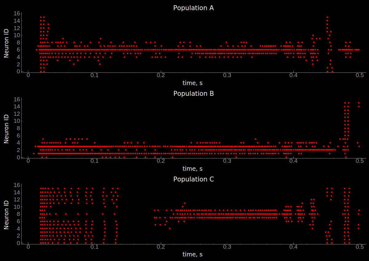
Network activity of a Threeway BuildingBlock.
Spike raster plot of the populations A, B and C encoding the relation A = B + C.
Teili2Genn
Using the already existing brian2genn we can generate GeNN code which can be executed on a nVidia graphics card.
Make sure to change the DPIsyn model located in teiliApps/equations/DPIsyn.py.
To be able to use brian2genn with TeiliNetwork change this line:
Iin{input_number}_post = I_syn * sign(weight) : amp (summed)
to
Iin{input_number}_post = I_syn * (-1 * (weight<0) + 1 * (weight>0)) : amp (summed)
Also move the following lines:
Iw = abs(weight) * baseweight                            : amp
I_gain = Io_syn*(I_syn<=Io_syn) + I_th*(I_syn>Io_syn)    : amp
Itau_syn = Io_syn*(I_syn<=Io_syn) + I_tau*(I_syn>Io_syn) : amp
to the on_pre key, such that it looks like:
'on_pre': """
     Iw = abs(weight) * baseweight                            : amp
     I_gain = Io_syn*(I_syn<=Io_syn) + I_th*(I_syn>Io_syn)    : amp
     Itau_syn = Io_syn*(I_syn<=Io_syn) + I_tau*(I_syn>Io_syn) : amp
     I_syn += Iw * w_plast * I_gain / (Itau_syn * ((I_gain/I_syn)+1))
     """,
Attention
If you don’t change the model GeNN can’t run its code generation routines as Subexpressions are not supported.
After you made the change in teiliApps/equations/DPIsyn.py you can run the teili2genn_tutorial.py located in teiliApps/tutorials/.
The TeiliNetwork is the same as in neuron_synapse_tutorial but with the specific commands to use the genn-backend.
WTA live plot
The point of this tutorial is to demonstrate the live plot and parameter gui. They are imported as follows:
from teili.tools.live import ParameterGUI, PlotGUI
We can add a live plot by instantiating a PlotGUI as follows:
plot_gui = PlotGUI(data=neuron_group.statevariable)
Currently this only supports plotting a statevariable of a neuron or synapse group or subgroup with a line plot.
The parameter GUI is instantiated as follows:
param_gui = ParameterGUI(net=Net)
param_gui.add_params(parameters=[synapse_group.weight, neuron_group.state_variable])
param_gui.show_gui()
Make sure, you specify the state variables that you change in the GUI as (shared), so that they are the same for the whole group. Or, as shown here in the tutorial, you can also just add a new state variable and copy over the value (or do other things with it) in a run_regularly:
syn_in_ex.add_state_variable('guiweight', unit=1, shared=True, constant=False, changeInStandalone=False)
syn_in_ex.guiweight = 400
syn_in_ex.run_regularly("weight = guiweight", dt=1 * ms)
Note
The brian2 simulator is not made for real time plotting. This currently only works with numpy code generation and timestep length can vary.
DVS visualizer
The point of this tutorial is to demonstrate how you can use the Plotter2d class to make a plot of 2d neural activity or DVS recordings. In this tutorials, you are asked to provide a path for 2 .aedat or .npz files that are then plotted next to each other.
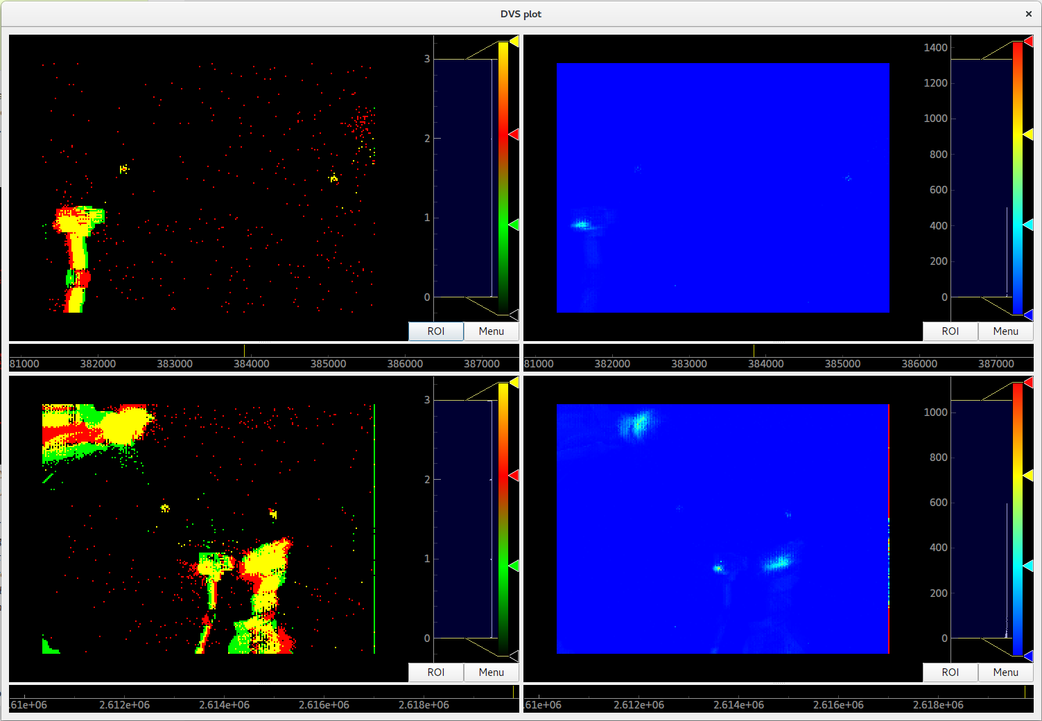
On the left side, the on and off events of the two loaded DVS files are shown.
On the right side, a (temporally) filtered version of the dvs events is shown.
We use QtGui.QGridLayout to arrange the ImageViews that we get from the Plotter in a grid.
Sequence learning standalone
The point of this tutorial is to demonstrate the c++ standalone codegeneration and replacing of parameters in the c++ code
so we can run the same compiled standalone program several times with different parameters.
The tutorial re-implements the sequence learning architecture described by Kreiser et al. 2018.
The full tutorial can be found at ~/teiliApps/tutorials/sequence_learning_standalone_tutorial.py
After the standalone_params (that can be passed to the compiled program) are defined, the network is built:
seq_net.standalone_params = standalone_params
seq_net.build()
Then it can be run several times with different parameters (without recompiling) and the results can be plotted in between.
seq_net.run(duration * second, standaloneParams=standalone_params)
This can be used if you have networks that you need to run very often with different parameters in a loop.