Tutorials
Welcome to teili, a modular python-based framework for developing, testing and visualization of neural algorithms. Before going through our tutorials we highly recommend doing the tutorials provided by Brian2
Dynamic model generation vs. static model import
Working with the dynamic model generation method
See an example for how to import model classes defined in models.neuron_models and models.synapse_models below.
from teili.core.groups import Neurons, Connections

from teili.models.neuron_models import DPI as neuron_model
from teili.models.synapse_models import DPISyn as syn_model

test_neuron1 = Neurons(N=2,
                       equation_builder=neuron_model(num_inputs=2),
                       name="test_neuron1", verbose=True)

test_neuron2 = Neurons(N=2,
                       equation_builder=neuron_model(num_inputs=2),
                       name="test_neuron2",verbose=True)

test_synapse = Connections(test_neuron1, test_neuron2,
                           equation_builder=syn_model,
                           name="test_synapse", verbose=True)
If you want to see a less detailed report on which equations were used during the generation you can set verbose=False.
Note
The Neurons class a num_inputs property. This allows the user to define how many different afferent connections this particular neuron population has to expect. The default is set to 1. Do not define more inputs than you expect.
Working with the static model import method
If you prefer to use neuron and synapse models statically specified in a file you can import default models from teiliApps/equations directory using the import_eq method. You can manually tweak these models and also generate your own models. For more information please have a look at the EquationBuilder.
import os
from teili.core.groups import Neurons, Connections
from teili.models.builder.neuron_equation_builder import NeuronEquationBuilder
from teili.models.builder.synapse_equation_builder import SynapseEquationBuilder

path = os.path.expanduser("~")
model_path = os.path.join(path, "teiliApps", "equations", "")

my_neuron_model = NeuronEquationBuilder.import_eq(
        model_path + 'DPI.py', num_inputs=2)

my_synapse_model = SynapseEquationBuilder.import_eq(
        model_path + 'DPISyn.py')

test_neuron1 = Neurons(N=2,
                       equation_builder=my_neuron_model,
                       name="test_neuron1")
test_neuron2 = Neurons(N=2,
                       equation_builder=my_neuron_model,
                       name="test_neuron2")

test_synapse = Connections(test_neuron1, test_neuron2,
                           equation_builder=my_synapse_model,
                           name="test_synapse")
If you want to see a more detailed report on which equations were used during the generation you can set verbose=True, such that it looks like this
test_neuron1 = Neurons(N=2,
                       equation_builder=my_neuron_model,
                       name="test_neuron1", verbose=True)
Neuron & Synapse tutorial
We created a simple tutorial of how to simulate a small neural network either using the EquationBuilder.
The complete tutorial is located in teiliApps/tutorials/neuron_synapse_tutorial.py.
Import relevant libraries
First we import all required libraries
from pyqtgraph.Qt import QtGui
import pyqtgraph as pg
import numpy as np

from Brian2 import ms, pA, nA, prefs,\
        SpikeMonitor, StateMonitor,\
        SpikeGeneratorGroup

from teili.core.groups import Neurons, Connections
from teili import TeiliNetwork
from teili.models.neuron_models import DPI as neuron_model
from teili.models.synapse_models import DPISyn as syn_model
from teili.models.parameters.dpi_neuron_param import parameters as neuron_model_param

from teili.tools.visualizer.DataViewers import PlotSettings
from teili.tools.visualizer.DataControllers import Rasterplot, Lineplot
We now can define the target for the code generation. Typically we use the numpy backend.
For more details on how to run your code more efficient and faster have a look at brian’s standalone mode
prefs.codegen.target = "numpy"
Defining the input stimulus
We can now generate a simple input pattern using Brian2’s SpikeGeneratorGroup
input_timestamps = np.asarray([1, 3, 4, 5, 6, 7, 8, 9]) * ms
input_indices = np.asarray([0, 0, 0, 0, 0, 0, 0, 0])
input_spikegenerator = SpikeGeneratorGroup(1, indices=input_indices,
                                           times=input_timestamps, name='gtestInp')
After defining the input group, we can build a TeiliNetwork.
Defining the network
Net = TeiliNetwork()

test_neurons1 = Neurons(N=2,
                        equation_builder=neuron_model(num_inputs=2),
                        name="test_neurons1")

test_neurons2 = Neurons(N=2,
                        equation_builder=neuron_model(num_inputs=2),
                        name="test_neurons2")


input_synapse = Connections(input_spikegenerator, test_neurons1,
                            equation_builder=syn_model(),
                            name="input_synapse")
input_synapse.connect(True)

test_synapse = Connections(test_neurons1, test_neurons2,
                           equation_builder=syn_model(),
                           name="test_synapse")
test_synapse.connect(True)
After initialising the populations of Neurons and connecting them via synaptic Connections, we can set model parameters.
Setting parameters
Note that parameters are set by default. This example only shows how you would need to go about if you want to set non-default (user defined) parameters.
Example parameter dictionaries can be found teili/models/parameters.
You can change all the parameters like this after creation of the Neurons or Connections.
# Example of how to set parameters, saved as a dictionary
test_neurons1.set_params(neuron_model_param)
test_neurons2.set_params(neuron_model_param)

# Example of how to set a single parameter
test_neurons1.refP = 1 * ms
test_neurons2.refP = 1 * ms

if 'Imem' in neuron_model().keywords['model']:
        input_synapse.weight = 5000
        test_synapse.weight = 800
        test_neurons1.Iconst = 10 * nA
elif 'Vm' in neuron_model().keywords['model']:
        input_synapse.weight = 1.5
        test_synapse.weight = 8.0
        test_neurons1.Iconst = 3 * nA
Note
The if condition is only there for convenience of the user to run our tutorial and switch between voltage- or current-based models. Normally, you have either current or voltage-based models in your simulation, thus you will not need the if condition.
Attention
The weight of a given Connection is multiplied with the baseweight, which is currently initialised to 7 pA by default for the DPI synapse model. In order to elicit an output spike in response to a single SpikeGenerator input spike the weight must be greater than 3250.
Now our simple spiking neural network is defined. In order to visualize what is happening during the simulation we need to monitor the spiking behaviour of our neurons and other state variables of neurons and synapses.
Defining monitors
spikemon_input = SpikeMonitor(
        input_spikegenerator, name='spikemon_input')
spikemon_test_neurons1 = SpikeMonitor(
        test_neurons1, name='spikemon_test_neurons1')
spikemon_test_neurons2 = SpikeMonitor(
        test_neurons2, name='spikemon_test_neurons2')

statemon_input_synapse = StateMonitor(
        input_synapse, variables='I_syn',
        record=True, name='statemon_input_synapse')

statemon_test_synapse = StateMonitor(
        test_synapse, variables='I_syn',
        record=True, name='statemon_test_synapse')

if 'Imem' in neuron_model().keywords['model']:
        statemon_test_neurons1 = StateMonitor(test_neurons1,
                                              variables=["Iin", "Imem", "Iahp"],
                                              record=[0, 1],
                                              name='statemon_test_neurons1')

        statemon_test_neurons2 = StateMonitor(test_neurons2,
                                              variables=['Imem'],
                                              record=0,
                                              name='statemon_test_neurons2')


elif 'Vm' in neuron_model().keywords['model']:
        statemon_test_neurons1 = StateMonitor(test_neurons1,
                                              variables=["Iin", "Vm", "Iadapt"],
                                              record=[0, 1],
                                              name='statemon_test_neurons1')

        statemon_test_neurons2 = StateMonitor(test_neurons2,
                                              variables=['Vm'],
                                              record=0,
                                              name='statemon_test_neurons2')
Starting the simulation
We can now finally add all defined Neurons and Connections, as well as the monitors to our TeiliNetwork and run the simulation.
Net.add(input_spikegenerator,
        test_neurons1, test_neurons2,
        input_synapse, test_synapse,
        spikemon_input, spikemon_test_neurons1,
        spikemon_test_neurons2,
        statemon_test_neurons1, statemon_test_neurons2,
        statemon_test_synapse, statemon_input_synapse)

duration = 500
Net.run(duration * ms)
Using statically defined models instead
If you, however, prefer to use the equation files located in teiliApps/equations/, you need to change the way the neurons and synapses are defined. The only thing that changes from the example above is the import and neuron/synapse group definition. The complete tutorial can be found in teiliApps/tutorials/neuron_synapse_import_eq_tutorial.py.
import os
from teili.models.builder.neuron_equation_builder import NeuronEquationBuilder
from teili.models.builder.synapse_equation_builder import SynapseEquationBuilder

# For this example you must first run models/neuron_models.py and synapse_models.py,
# which will create the equation template. This will be stored in models/equations
# Building neuron objects

path = os.path.expanduser("~")
model_path = os.path.join(path, "teiliApps", "equations", "")

builder_object1 = NeuronEquationBuilder.import_eq(
        model_path + 'DPI.py', num_inputs=2)
builder_object2 = NeuronEquationBuilder.import_eq(
        model_path + 'DPI.py', num_inputs=2)

builder_object3 = SynapseEquationBuilder.import_eq(
        model_path + 'DPISyn.py')
builder_object4 = SynapseEquationBuilder.import_eq(
        model_path + 'DPISyn.py')

test_neurons1 = Neurons(2, equation_builder=builder_object1, name="test_neurons1")
test_neurons2 = Neurons(2, equation_builder=builder_object2, name="test_neurons2")

input_synapse = Connections(input_spikegenerator, test_neurons1,
                            equation_builder=builder_object3,
                            name="input_synapse", verbose=False)
input_synapse.connect(True)
test_synapse = Connections(test_neurons1, test_neurons2,
                           equation_builder=builder_object4, name="test_synapse")
test_synapse.connect(True)
The way parameters are set remains the same.
Visualising the networks activity
In order to visualize the behaviour the example script also plots a couple of spike and state monitors.
For a full tutorial of how use teili’s Visualizer class please refer to our visualiser tutorial
app = QtGui.QApplication.instance()
if app is None:
    app = QtGui.QApplication(sys.argv)
else:
    print('QApplication instance already exists: %s' % str(app))

pg.setConfigOptions(antialias=True)
labelStyle = {'color': '#FFF', 'font-size': 12}
MyPlotSettings = PlotSettings(fontsize_title=labelStyle['font-size'],
                              fontsize_legend=labelStyle['font-size'],
                              fontsize_axis_labels=10,
                              marker_size=7)

win = pg.GraphicsWindow()
win.resize(2100, 1200)
win.setWindowTitle('Simple Spiking Neural Network')

p1 = win.addPlot(title="Input spike generator")
p2 = win.addPlot(title="Input synapses")
win.nextRow()
p3 = win.addPlot(title='Intermediate test neurons 1')
p4 = win.addPlot(title="Test synapses")
win.nextRow()
p5 = win.addPlot(title="Rasterplot of output test neurons 2")
p6 = win.addPlot(title="Output test neurons 2")


# Spike generator
Rasterplot(MyEventsModels=[spikemon_input],
                     MyPlotSettings=MyPlotSettings,
                     time_range=[0, duration],
                     neuron_id_range=None,
                     title="Input spike generator",
                     xlabel='Time (ms)',
                     ylabel="Neuron ID",
                     backend='pyqtgraph',
                     mainfig=win,
                     subfig_rasterplot=p1,
                     QtApp=app,
                     show_immediately=False)

# Input synapses
Lineplot(DataModel_to_x_and_y_attr=[(statemon_input_synapse, ('t', 'I_syn'))],
                   MyPlotSettings=MyPlotSettings,
                   x_range=[0, duration],
                   title="Input synapses",
                   xlabel="Time (ms)",
                   ylabel="EPSC (A)",
                   backend='pyqtgraph',
                   mainfig=win,
                   subfig=p2,
                   QtApp=app,
                   show_immediately=False)

# Intermediate neurons
if hasattr(statemon_test_neurons1, 'Imem'):
    MyData_intermed_neurons = [(statemon_test_neurons1, ('t', 'Imem'))]
if hasattr(statemon_test_neurons1, 'Vm'):
    MyData_intermed_neurons = [(statemon_test_neurons1, ('t', 'Vm'))]

i_current_name = 'Imem' if 'Imem' in neuron_model().keywords['model'] else 'Vm'
Lineplot(DataModel_to_x_and_y_attr=MyData_intermed_neurons,
                   MyPlotSettings=MyPlotSettings,
                   x_range=[0, duration],
                   title='Intermediate test neurons 1',
                   xlabel="Time (ms)",
                   ylabel=i_current_name,
                   backend='pyqtgraph',
                   mainfig=win,
                   subfig=p3,
                   QtApp=app,
                   show_immediately=False)

# Output synapses
Lineplot(DataModel_to_x_and_y_attr=[(statemon_test_synapse, ('t', 'I_syn'))],
                   MyPlotSettings=MyPlotSettings,
                   x_range=[0, duration],
                   title="Test synapses",
                   xlabel="Time (ms)",
                   ylabel="EPSC (A)",
                   backend='pyqtgraph',
                   mainfig=win,
                   subfig=p4,
                   QtApp=app,
                   show_immediately=False)


Rasterplot(MyEventsModels=[spikemon_test_neurons2],
                     MyPlotSettings=MyPlotSettings,
                     time_range=[0, duration],
                     neuron_id_range=None,
                     title="Rasterplot of output test neurons 2",
                     xlabel='Time (ms)',
                     ylabel="Neuron ID",
                     backend='pyqtgraph',
                     mainfig=win,
                     subfig_rasterplot=p5,
                     QtApp=app,
                     show_immediately=False)

if hasattr(statemon_test_neurons2, 'Imem'):
    MyData_output = [(statemon_test_neurons2, ('t','Imem'))]
if hasattr(statemon_test_neurons2, 'Vm'):
    MyData_output = [(statemon_test_neurons2, ('t','Vm'))]

Lineplot(DataModel_to_x_and_y_attr=MyData_output,
                   MyPlotSettings=MyPlotSettings,
                   x_range=[0, duration],
                   title="Output test neurons 2",
                   xlabel="Time (ms)",
                   ylabel="%s" %i_current_name,
                   backend='pyqtgraph',
                   mainfig=win,
                   subfig=p6,
                   QtApp=app,
                   show_immediately=False)

app.exec()
In both cases of model definition (rather dynamic model generation or static model import) the resulting figure should look like this:
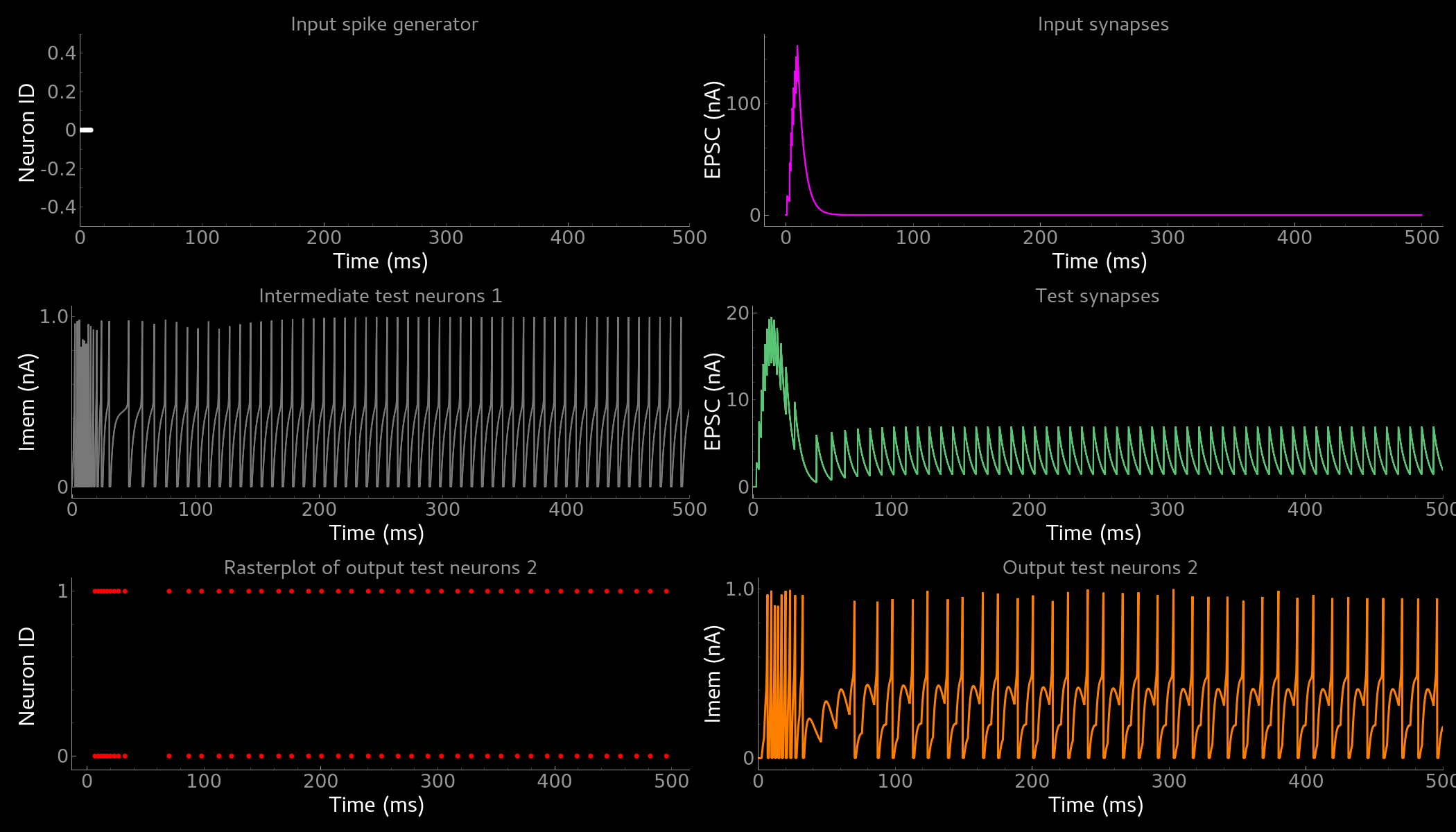
Simple neuron and networks dynamics.
Top left) Spike raster plot of the SpikeGeneratorGroup. Top right) Excitatory post-synaptic current in nA of the input synapse over time. Middle left) Membrane current of the DPI neuron in nA over time. Middle right) Excitatory post-synaptic current in nA of the synapse between neuron populations over time. Bottom left) Spike raster plot of the second neuron population. Bottom right) Membrane current of the second population in nA over time.
Synaptic kernels tutorial
In teili we provide synaptic models that modify the shape of synaptic currents, which we call kernels. Here we provide a tutorial of how to use them and how they look when applied together with a neuron model.
The first steps are the same as in the previous tutorial.
The tutorial is located in teiliApps/tutorials/synaptic_kernels_tutorial.py.
We first import all required libraries:
from pyqtgraph.Qt import QtGui, QtCore
import pyqtgraph as pg
import numpy as np

from brian2 import second, ms, prefs,\
        SpikeMonitor, StateMonitor,\
        SpikeGeneratorGroup

from teili.core.groups import Neurons, Connections
from teili import TeiliNetwork
from teili.models.neuron_models import DPI as neuron_model
from teili.models.synapse_models import Alpha, Resonant, DPISyn
from teili.models.parameters.dpi_neuron_param import parameters as neuron_model_param

from teili.tools.visualizer.DataViewers import PlotSettings
from teili.tools.visualizer.DataModels import  StateVariablesModel
from teili.tools.visualizer.DataControllers import Lineplot
We define the target for the code generation. As in the previous example we use the numpy backend.
prefs.codegen.target = "numpy"
We define a simple input pattern using Brian2’s SpikeGeneratorGroup. This will consist of two neurons, one will send excitatory and the other inhibitory spikes.
input_timestamps = np.asarray([1, 1.5, 1.8, 2.0, 2.0, 2.3, 2.5, 3]) * ms
input_indices = np.asarray([0, 1, 0, 1, 0, 1, 0, 1])
input_spikegenerator = SpikeGeneratorGroup(2, indices=input_indices,
                                times=input_timestamps, name='gtestInp')
We now build a TeiliNetwork.
Net = TeiliNetwork()
In this tutorial we will show three kernels, therefore we have created three different neurons. The first one will receive synapses with an Alpha kernel shape, the second will receive synapses with a Resonant kernel shape and the third one will receive a synapse which models the DPI synapse model, which has an exponential decay shape. Note that a single neuron can receive synapses with different kernels at the same time. Here we split them for better visualisation.
test_neurons1 = Neurons(1,
equation_builder=neuron_model(num_inputs=2), name="test_neurons")

test_neurons1.set_params(neuron_model_param)
test_neurons1.refP = 1 * ms

test_neurons2 = Neurons(1,
equation_builder=neuron_model(num_inputs=2), name="test_neurons2")

test_neurons2.set_params(neuron_model_param)
test_neurons2.refP = 1 * ms

test_neurons3 = Neurons(1,
equation_builder=neuron_model(num_inputs=2), name="test_neurons3")

test_neurons3.set_params(neuron_model_param)
test_neurons3.refP = 1 * ms
Note
We are using the DPI neuron model for this tutorial but the synaptic model is independent of the neuron’s model and therefore other neuron models can be used.
We already set the parameters for our neuron model. As explained above, we can set the standard parameters from a dictionary but also change single parameters as in this example with the refractory period.
Now we specify the connections. The synaptic models are Alpha, Resonant and DPI.
syn_alpha = Connections(input_spikegenerator, test_neurons1,
                     equation_builder=Alpha(), name="test_syn_alpha", verbose=False)
syn_alpha.connect(True)

syn_resonant = Connections(input_spikegenerator, test_neurons2,
                 equation_builder=Resonant(), name="test_syn_resonant", verbose=False)
syn_resonant.connect(True)

syn_dpi = Connections(input_spikegenerator, test_neurons3,
                 equation_builder=DPISyn(), name="test_syn_dpi", verbose=False)
syn_dpi.connect(True)
We set the parameters for the synapses. In this case, we specify that the first neuron in the SpikeGenerator will have an excitatory effect (weight>0) and the second neuron will have an inhibitory effect (weight<0) on the post-synaptic neuron.
syn_alpha.weight = np.asarray([10,-10])
syn_resonant.weight = np.asarray([10,-10])
syn_dpi.weight = np.asarray([10,-10])
Attention
The weight of a given Connection is multiplied with the baseweight, which is currently initialised to 7 pA by default for the DPI synapse model. In order to elicit an output spike in response to a single SpikeGenerator input spike the weight must be greater than 3250.
Now our simple spiking neural network is defined. In order to visualize what is happening during the simulation
we need to monitor the spiking behaviour of our Neurons and other state variables of our Neurons and Connections.
spikemon_inp = SpikeMonitor(input_spikegenerator, name='spikemon_inp')
statemon_syn_alpha = StateMonitor(syn_alpha, variables='I_syn',
                                  record=True, name='statemon_syn_alpha')
statemon_syn_resonant = StateMonitor(syn_resonant,variables='I_syn',
                                     record=True, name='statemon_syn_resonant')
statemon_syn_dpi = StateMonitor(syn_dpi, variables='I_syn',
                                record=True, name='statemon_syn_dpi')
statemon_test_neuron1 = StateMonitor(test_neurons1, variables=['Iin'],
                                     record=0, name='statemon_test_neuron1')
statemon_test_neuron2 = StateMonitor(test_neurons2, variables=['Iin'],
                                     record=0, name='statemon_test_neuron2')
statemon_test_neuron3 = StateMonitor(test_neurons3, variables=['Iin'],
                                     record=0, name='statemon_test_neuron3')
We can now finally add all defined Neurons and Connections and also the monitors to our TeiliNetwork and run the simulation.
Net.add(input_spikegenerator,
        test_neurons1,
        test_neurons2,
        test_neurons3,
        syn_alpha,
        syn_resonant,
        syn_dpi,
        spikemon_inp,
        statemon_syn_alpha,
        statemon_syn_resonant,
        statemon_syn_dpi,
        statemon_test_neuron1,
        statemon_test_neuron2,
        statemon_test_neuron3)

duration = 0.010
Net.run(duration * second)
In order to visualize the behaviour, the example script also plots a couple of spike and state monitors.
app = QtGui.QApplication.instance()
if app is None:
    app = QtGui.QApplication(sys.argv)
else:
    print('QApplication instance already exists: %s' % str(app))

pg.setConfigOptions(antialias=True)
labelStyle = {'color': '#FFF', 'font-size': 12}
MyPlotSettings = PlotSettings(fontsize_title=labelStyle['font-size'],
                              fontsize_legend=labelStyle['font-size'],
                              fontsize_axis_labels=10,
                              marker_size=7)

win = pg.GraphicsWindow(title='Kernels Simulation')
win.resize(900, 600)
win.setWindowTitle('Simple SNN')

p1 = win.addPlot()
p2 = win.addPlot()
win.nextRow()
p3 = win.addPlot()
p4 = win.addPlot()
win.nextRow()
p5 = win.addPlot()
p6 = win.addPlot()

# Alpha kernel synapse
data = statemon_syn_alpha.I_syn.T
data[:, 1] *= -1.
datamodel_syn_alpha = StateVariablesModel(state_variable_names=['I_syn'],
                                state_variables=[data],
                                state_variables_times=[statemon_syn_alpha.t])
Lineplot(DataModel_to_x_and_y_attr=[(datamodel_syn_alpha, ('t_I_syn', 'I_syn'))],
         MyPlotSettings=MyPlotSettings,
         x_range=(0, duration),
         y_range=None,
         title='Alpha Kernel Synapse',
         xlabel='Time (s)',
         ylabel='Synaptic current I (A)',
         backend='pyqtgraph',
         mainfig=win,
         subfig=p1,
         QtApp=app)
for i, data in enumerate(np.asarray(spikemon_inp.t)):
    vLine = pg.InfiniteLine(pen=pg.mkPen(color=(200, 200, 255),
                style=QtCore.Qt.DotLine),pos=data, angle=90, movable=False,)
    p1.addItem(vLine, ignoreBounds=True)

# Neuron response
Lineplot(DataModel_to_x_and_y_attr=[(statemon_test_neuron1, ('t', 'Iin'))],
         MyPlotSettings=MyPlotSettings,
         x_range=(0, duration),
         y_range=None,
         title='Neuron response',
         xlabel='Time (s)',
         ylabel='Membrane current I_mem (A)',
         backend='pyqtgraph',
         mainfig=win,
         subfig=p2,
         QtApp=app)

# Resonant kernel synapse
data = statemon_syn_resonant.I_syn.T
data[:, 1] *= -1.
datamodel_syn_resonant = StateVariablesModel(state_variable_names=['I_syn'],
                                state_variables=[data],
                                state_variables_times=[statemon_syn_resonant.t])

Lineplot(DataModel_to_x_and_y_attr=[(datamodel_syn_resonant, ('t_I_syn','I_syn'))],
         MyPlotSettings=MyPlotSettings,
         x_range=(0, duration),
         y_range=None,
         title='Resonant Kernel Synapse',
         xlabel='Time (s)',
         ylabel='Synaptic current I (A)',
         backend='pyqtgraph',
         mainfig=win,
         subfig=p3,
         QtApp=app)
for i, data in enumerate(np.asarray(spikemon_inp.t)):
    vLine = pg.InfiniteLine(pen=pg.mkPen(color=(200, 200, 255),
                style=QtCore.Qt.DotLine),pos=data, angle=90, movable=False,)
    p3.addItem(vLine, ignoreBounds=True)

# Neuron response
Lineplot(DataModel_to_x_and_y_attr=[(statemon_test_neuron2, ('t', 'Iin'))],
         MyPlotSettings=MyPlotSettings,
         x_range=(0, duration),
         y_range=None,
         title='Neuron response',
         xlabel='Time (s)',
         ylabel='Membrane current I_mem (A)',
         backend='pyqtgraph',
         mainfig=win,
         subfig=p4,
         QtApp=app)

# DPI synapse
data = statemon_syn_dpi.I_syn.T
data[:, 1] *= -1.
datamodel_syn_dpi = StateVariablesModel(state_variable_names=['I_syn'],
                                state_variables=[data],
                                state_variables_times=[statemon_syn_dpi.t])

Lineplot(DataModel_to_x_and_y_attr=[(datamodel_syn_dpi, ('t_I_syn','I_syn'))],
         MyPlotSettings=MyPlotSettings,
         x_range=(0, duration),
         y_range=None,
         title='DPI Synapse',
         xlabel='Time (s)',
         ylabel='Synaptic current I (A)',
         backend='pyqtgraph',
         mainfig=win,
         subfig=p5,
         QtApp=app)
for i, data in enumerate(np.asarray(spikemon_inp.t)):
    vLine = pg.InfiniteLine(pen=pg.mkPen(color=(200, 200, 255),
                style=QtCore.Qt.DotLine),pos=data, angle=90, movable=False,)
    p5.addItem(vLine, ignoreBounds=True)

# Neuron response
Lineplot(DataModel_to_x_and_y_attr=[(statemon_test_neuron3, ('t', 'Iin'))],
         MyPlotSettings=MyPlotSettings,
         x_range=(0, duration),
         y_range=None,
         title='Neuron response',
         xlabel='Time (s)',
         ylabel='Membrane current I_mem (A)',
         backend='pyqtgraph',
         mainfig=win,
         subfig=p6,
         QtApp=app,
         show_immediately=True)
The synaptic current is always positive, the negative effect is observed in the Iin of the neuron. To better visualize the synapse dynamics, we have multiplied the I_syn of the inhibitory synapse by -1. The resulting figure should look like this:
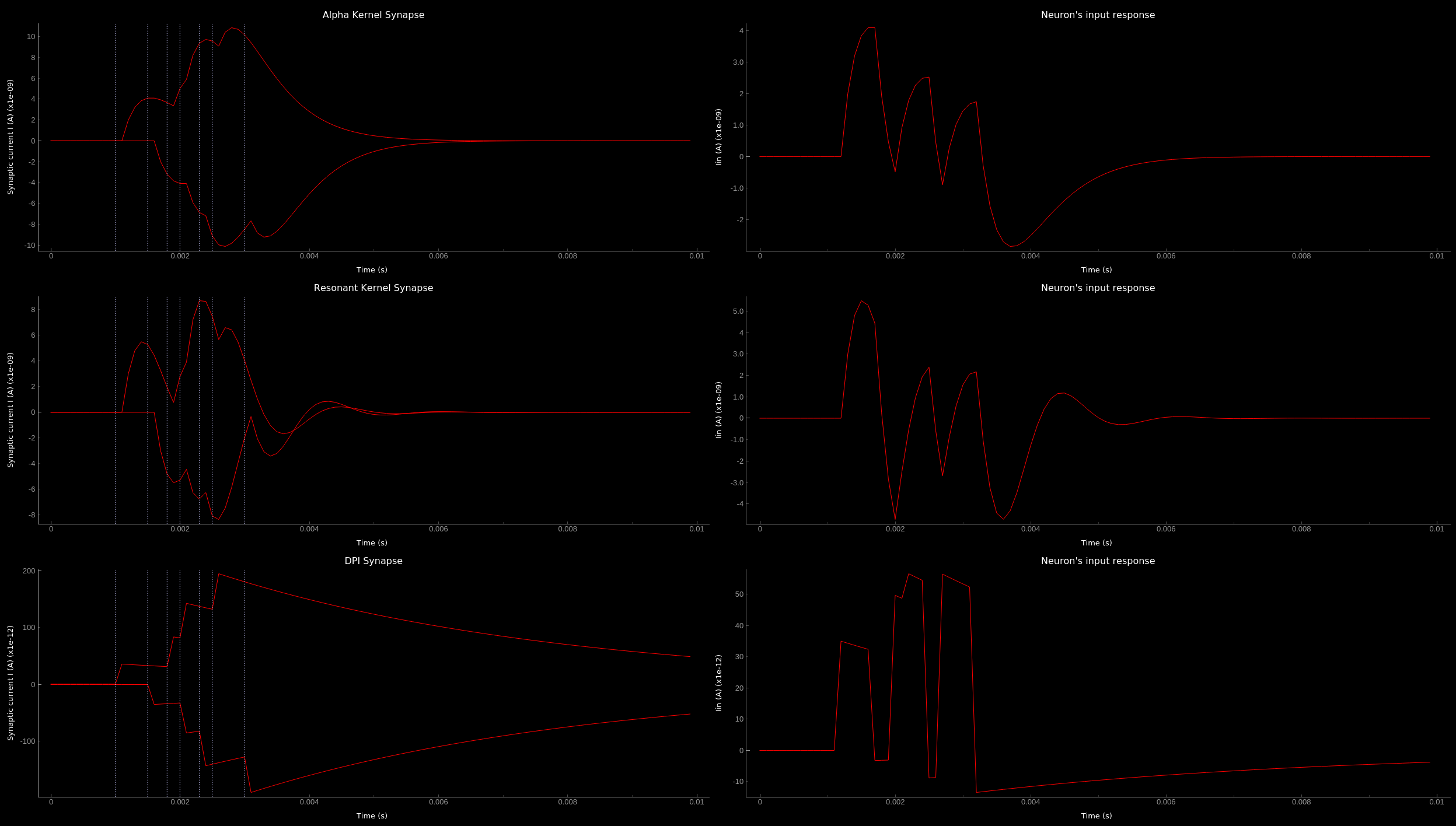
Synaptic kernels. Synaptic current traces for different synaptic kernels and the resulting effect on Iin. Alpha (top), resonant (middle) and DPI (bottom) synaptic kernel is shown.
Winner-takes-all tutorial
teili not only offers simple neuron-synapse models, but rather aims to provide high-level description of neuronal algorithms which can be formalised as scalable building blocks.
One example BuildingBlock is the winner-takes-all (WTA) network.
To show the basic interface of how to use a WTA network we start with the imports.
The original file can be found in teiliApps/tutorials/wta_tutorial.py
Note
For instructions on how to design a novel BuildingBlock please refer to BuildingBlock development
import os
import sys
import numpy as np
import matplotlib.pyplot as plt
from collections import OrderedDict
from pyqtgraph.Qt import QtGui
import pyqtgraph as pg

import scipy
from scipy import ndimage

from Brian2 import prefs, ms, pA, StateMonitor, SpikeMonitor,\
        device, set_device,\
        second, msecond, defaultclock

from teili.building_blocks.wta import WTA
from teili.core.groups import Neurons, Connections
from teili.stimuli.testbench import WTA_Testbench
from teili import TeiliNetwork
from teili.models.synapse_models import DPISyn

from teili.tools.visualizer.DataControllers import Rasterplot
Now we can define the code generation backend.
Here the user can either use the standard numpy backend, or by setting run_as_standalone = True the code will be compiled as C++ code before it is executed.
Note
To run the WTA BuildingBlock in standalone mode please refer to our standalone tutorial which is located in teiliApps/tutorials/wta_standalone_tutorial.py.
prefs.codegen.target = 'numpy'
run_as_standalone = False

if run_as_standalone:
        standaloneDir = os.path.expanduser('~/WTA_standalone')
        set_device('cpp_standalone', directory=standaloneDir, build_on_run=False)
        device.reinit()
        device.activate(directory=standaloneDir, build_on_run=False)
        prefs.devices.cpp_standalone.openmp_threads = 2
We need to define two hyperparameters of our WTA and to illustrate its working behaviour, we initialize an instance of a stimulus test class specifically designed for WTA’s.
num_neurons = 50
num_input_neurons = num_neurons
num_inh_neurons = 40

Net = TeiliNetwork()
duration = 500
testbench = WTA_Testbench()
In contrast to the simple spiking network discussed so far, BuildingBlocks are a bit more complicated.
When we generate our BuildingBlock, we need to pass specific parameters, which set internal synaptic weights, connectivity kernels and connectivity probabilities.
For more information see BuildingBlocks documentation and the source code, respectively.
To do so we define a dictionary, which is passed to the BuildingBlock class.
Feel free to change the parameters to see what effect it has on the stability and signal-to-noise ratio.
wta_params = {'we_inp_exc': 900,
              'we_exc_inh': 500,
              'wi_inh_exc': -550,
              'we_exc_exc': 650,
              'sigm': 2,
              'rp_exc': 3 * ms,
              'rp_inh': 1 * ms,
              'ei_connection_probability': 0.7,
              }
We can define our network structure and connect the different inputs to the WTA network.
test_WTA = WTA(name='test_WTA', dimensions=1,
              num_neurons=num_neurons,
              num_inh_neurons=num_inh_neurons,
              num_input_neurons=num_input_neurons,
              num_inputs=2, block_params=wta_params,
              spatial_kernel="kernel_gauss_1d")

testbench.stimuli(num_neurons=num_input_neurons,
                  dimensions=1,
                  start_time=100, end_time=duration)

testbench.background_noise(num_neurons=num_input_neurons, rate=10)

test_WTA.spike_gen.set_spikes(
        indices=testbench.indices, times=testbench.times * ms)

noise_syn = Connections(testbench.noise_input,
                        test_WTA._groups['n_exc'],
                        equation_builder=DPISyn(),
                        name="noise_syn")
noise_syn.connect("i==j")
Before we can run the simulation we need to set bias parameter.
Attention
The weight of a given Connection is multiplied with the baseweight, which is currently initialised to 7 pA by default for the DPI synapse model. In order to elicit an output spike in response to a single SpikeGenerator input spike the weight must be greater than 3250.
noise_syn.weight = 3000
Setting up monitors to track network activity and visualize it later.
statemon_wta_input = StateMonitor(test_WTA._groups['n_exc'],
                             ('Iin0', 'Iin1', 'Iin2', 'Iin3'),
                             record=True,
                             name='statemon_wta_input')

spikemonitor_wta_input = SpikeMonitor(
        test_WTA.spike_gen, name="spikemonitor_wta_input")
spikemonitor_noise = SpikeMonitor(
        testbench.noise_input, name="spikemonitor_noise")
Add all population and monitor objects to the network object and define standalone parameters, if you are using standalone mode.
Net.add(test_WTA, testbench.noise_input, noise_syn,
        statemon_wta_input, spikemonitor_noise, spikemonitor_wta_input)
Net.standalone_params.update({'test_WTA_Iconst': 1 * pA})

if run_as_standalone:
        Net.build()

standalone_params = OrderedDict([('duration', 0.7 * second),
                                 ('stestWTA_e_latWeight', 650),
                                 ('stestWTA_e_latSigma', 2),
                                 ('stestWTA_Inpe_weight', 900),
                                 ('stestWTA_Inhe_weight', 500),
                                 ('stestWTA_Inhi_weight', -550),
                                 ('test_WTA_refP', 1. * msecond),
                                 ('testWTA_Inh_refP', 1. * msecond)])

duration = standalone_params['duration'] / ms
Net.run(duration=duration * ms, standalone_params=standalone_params, report='text')
Now we can visualise the activity of our WTA network using our Visualizer.
win_wta = pg.GraphicsWindow(title="WTA")
win_wta.resize(2500, 1500)
win_wta.setWindowTitle("WTA")
p1 = win_wta.addPlot()
win_wta.nextRow()
p2 = win_wta.addPlot()
win_wta.nextRow()
p3 = win_wta.addPlot()

spikemonWTA = test_WTA.monitors['spikemon_exc']
spiketimes = spikemonWTA.t

Rasterplot(MyEventsModels = [spikemonitor_noise],
            time_range=(0, duration_s),
            title="Noise input",
            xlabel='Time (s)',
            ylabel=None,
            backend='pyqtgraph',
            mainfig=win_wta,
            subfig_rasterplot=p1)

Rasterplot(MyEventsModels=[spikemonWTA],
            time_range=(0, duration_s),
            title="WTA activity",
            xlabel='Time (s)',
            ylabel=None,
            backend='pyqtgraph',
            mainfig=win_wta,
            subfig_rasterplot=p2)

Rasterplot(MyEventsModels=[spikemonitor_input],
            time_range=(0, duration_s),
            title="Actual signal",
            xlabel='Time (s)',
            ylabel=None,
            backend='pyqtgraph',
            mainfig=win_wta,
            subfig_rasterplot=p3,
            show_immediately=True)
The resulting figure should look like this:
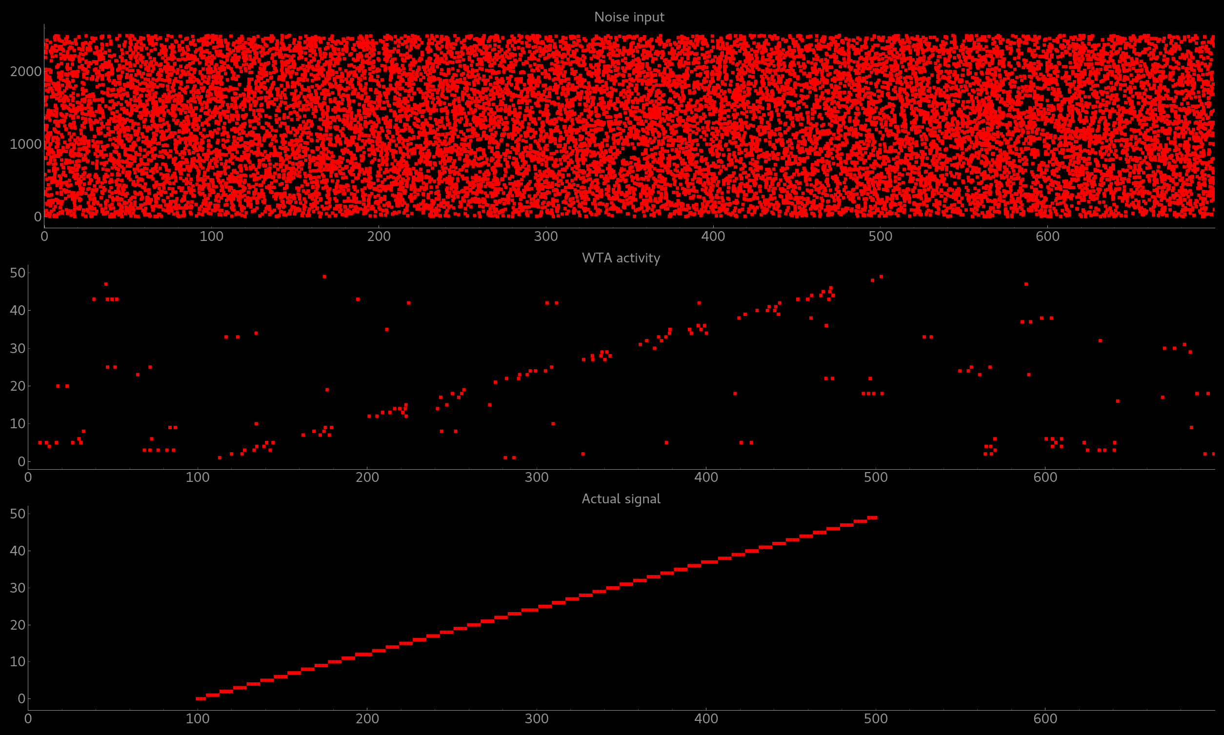
Simple signal restoration behaviour of soft WTA network.
The signal (shown in the bottom plot) is embededd in noise (top plot). The WTA restores the signal and effectively suppresses the noise (middle plot).
STDP tutorial
One key property of teili is that existing neuron/synapse models can easily be extended to provide additional functionality, such as extending a given synapse model with for example a Spike-Timing Dependent Plasticity (STDP) mechanism.
STDP is one mechanism which has been identified experimentally how neurons adjust their synaptic weight according to correlated firing patterns.
Feel free to read more about STDP.
The following tutorial can be found at teiliApps/tutorials/stdp_tutorial.py
If we want to add an activity dependent plasticity mechanism to our network we again start by importing the required packages.
from pyqtgraph.Qt import QtGui
import pyqtgraph as pg
import pyqtgraph.exporters
import numpy as np
import os

from Brian2 import ms, us, pA, prefs,\
        SpikeMonitor, StateMonitor, defaultclock

from teili.core.groups import Neurons, Connections
from teili import TeiliNetwork
from teili.models.neuron_models import DPI
from teili.models.synapse_models import DPISyn, DPIstdp
from teili.stimuli.testbench import STDP_Testbench

from teili.tools.visualizer.DataViewers import PlotSettings
from teili.tools.visualizer.DataModels import StateVariablesModel
from teili.tools.visualizer.DataControllers import Lineplot, Rasterplot
As before we can define the backend, as well as our TeiliNetwork:
prefs.codegen.target = "numpy"
defaultclock.dt = 50 * us
Net = TeiliNetwork()
Note that we changed the defaultclock.
This is usually helpful to prevent numerical integration error and to be sure that the network performs the desired computation. But keep in mind by decreasing the defaultclock.dt the simulation takes longer!
In the next step we will load a simple STDP-protocol from our STDP testbench, which provides us with pre-defined pre-post spikegenerators with specific delays between pre and post spiking activity.
stdp = STDP_Testbench()
pre_spikegenerator, post_spikegenerator = stdp.stimuli(isi=30)
Now we generate our test_neurons and connect via non-plastic synapses to our SpikeGeneratorGroups and via plastic synapses between them.
pre_neurons = Neurons(N=2,
                      equation_builder=DPI(num_inputs=1),
                      name='pre_neurons')

post_neurons = Neurons(N=2,
                       equation_builder=DPI(num_inputs=2),
                       name='post_neurons')


pre_synapse = Connections(pre_spikegenerator, pre_neurons,
                          equation_builder=DPISyn(),
                          name='pre_synapse')

post_synapse = Connections(post_spikegenerator, post_neurons,
                           equation_builder=DPISyn(),
                           name='post_synapse')

stdp_synapse = Connections(pre_neurons, post_neurons,
                           equation_builder=DPIstdp(),
                           name='stdp_synapse')

pre_synapse.connect(True)
post_synapse.connect(True)
We can now set the biases.
Note
Note that we define the temporal window of the STDP kernel using taupost and taupost bias. The learning rate, i.e. the amount of maximal weight change, is set by dApre.
pre_neurons.refP = 3 * ms
pre_neurons.Itau = 6 * pA

post_neurons.Itau = 6 * pA

pre_synapse.weight = 4000.

post_synapse.weight = 4000.

stdp_synapse.connect("i==j")
stdp_synapse.weight = 300.
stdp_synapse.I_tau = 10 * pA
stdp_synapse.dApre = 0.01
stdp_synapse.taupre = 3 * ms
stdp_synapse.taupost = 3 * ms
Now we define monitors, which are later use to visualize the STDP protocol and the respective weight change.
spikemon_pre_neurons = SpikeMonitor(pre_neurons, name='spikemon_pre_neurons')
statemon_pre_neurons = StateMonitor(pre_neurons, variables='Imem',
                                    record=0, name='statemon_pre_neurons')

spikemon_post_neurons = SpikeMonitor(
        post_neurons, name='spikemon_post_neurons')
statemon_post_neurons = StateMonitor(
        post_neurons, variables='Imem',
        record=0, name='statemon_post_neurons')

statemon_pre_synapse = StateMonitor(
        pre_synapse, variables=['I_syn'],
        record=0, name='statemon_pre_synapse')

statemon_post_synapse = StateMonitor(
        stdp_synapse,
        variables=['I_syn', 'w_plast', 'weight'],
        record=True,
        name='statemon_post_synapse')
We can now add all objects to our network and run the simulation.
Net.add(pre_spikegenerator, post_spikegenerator,
        pre_neurons, post_neurons,
        pre_synapse, post_synapse, stdp_synapse,
        spikemon_pre_neurons, spikemon_post_neurons,
        statemon_pre_neurons, statemon_post_neurons,
        statemon_pre_synapse, statemon_post_synapse)

duration = 2000
Net.run(duration * ms)
After the simulation is finished we can visualize the effect of the STDP synapse.
win_stdp = pg.GraphicsWindow(title="STDP Unit Test")
win_stdp.resize(2500, 1500)
win_stdp.setWindowTitle("Spike Time Dependent Plasticity")

p1 = win_stdp.addPlot()
win_stdp.nextRow()
p2 = win_stdp.addPlot()
win_stdp.nextRow()
p3 = win_stdp.addPlot()

text1 = pg.TextItem(text='Homoeostasis', anchor=(-0.3, 0.5))
text2 = pg.TextItem(text='Weak Pot.', anchor=(-0.3, 0.5))
text3 = pg.TextItem(text='Weak Dep.', anchor=(-0.3, 0.5))
text4 = pg.TextItem(text='Strong Pot.', anchor=(-0.3, 0.5))
text5 = pg.TextItem(text='Strong Dep.', anchor=(-0.3, 0.5))
text6 = pg.TextItem(text='Homoeostasis', anchor=(-0.3, 0.5))
p1.addItem(text1)
p1.addItem(text2)
p1.addItem(text3)
p1.addItem(text4)
p1.addItem(text5)
p1.addItem(text6)
text1.setPos(0, 0.5)
text2.setPos(0.300, 0.5)
text3.setPos(0.600, 0.5)
text4.setPos(0.900, 0.5)
text5.setPos(1.200, 0.5)
text6.setPos(1.500, 0.5)

Rasterplot(MyEventsModels=[spikemon_pre_neurons, spikemon_post_neurons],
            MyPlotSettings=PlotSettings(colors=['w', 'r']),
            time_range=(0, duration),
            neuron_id_range=(-1, 2),
            title="STDP protocol",
            xlabel="Time (s)",
            ylabel="Neuron ID",
            backend='pyqtgraph',
            mainfig=win_stdp,
            subfig_rasterplot=p1)

Lineplot(DataModel_to_x_and_y_attr=[(statemon_post_synapse, ('t', 'w_plast'))],
            MyPlotSettings=PlotSettings(colors=['g']),
            x_range=(0, duration),
            title="Plastic synaptic weight",
            xlabel="Time (s)",
            ylabel="Synpatic weight w_plast",
            backend='pyqtgraph',
            mainfig=win_stdp,
            subfig=p2)

datamodel = StateVariablesModel(state_variable_names=['I_syn'],
                                state_variables=[np.asarray(statemon_post_synapse.I_syn[1])],
                                state_variables_times=[np.asarray(statemon_post_synapse.t)])
Lineplot(DataModel_to_x_and_y_attr=[(datamodel, ('t_I_syn', 'I_syn'))],
            MyPlotSettings=PlotSettings(colors=['m']),
            x_range=(0, duration),
            title="Post synaptic current",
            xlabel="Time (s)",
            ylabel="Synapic current I (pA)",
            backend='pyqtgraph',
            mainfig=win_stdp,
            subfig=p3,
            show_immediately=True)
Attention
Please keep in mind that the spike times for the plasticity protocol are sampled randomly. The random sampling might lead to asymmetric weight updates.
The resulting figure should look like this:
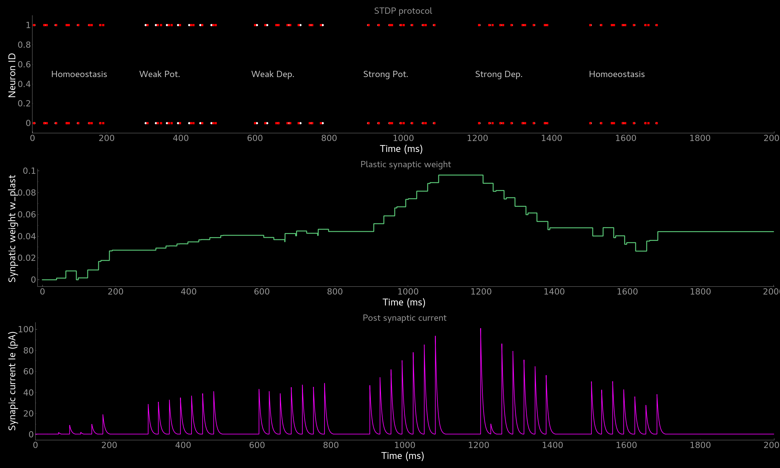
Effect of spike-time dependent plasticity (STDP) on synaptic weight and EPSC. Synaptic weight (middle) and resulting EPSC over time as a function of pre-post pairs of spikes. Homoeostasis, weak and strong potentation and depression are shown.
Visualizing plasticity kernel of STDP synapse
In order to better understand why the synaptic weight changes the way it does given the specific pre and post spike pairs we can visualize the STDP kernel. The following tutorial can be found at ~/teiliApps/tutorials/stdp_kernel_tutorial.py
We start again by importing the required dependencies.
from Brian2 import ms, prefs, SpikeMonitor, run
from pyqtgraph.Qt import QtGui
import pyqtgraph as pg
import matplotlib.pyplot as plt
import numpy as np

from teili.core.groups import Neurons, Connections
from teili.models.synapse_models import DPIstdp

from teili.tools.visualizer.DataViewers import PlotSettings
from teili.tools.visualizer.DataModels import StateVariablesModel
from teili.tools.visualizer.DataControllers import Lineplot, Rasterplot
We define the simulation and visualization backend. And specify explicitly the font used by the visualization.
prefs.codegen.target = "numpy"
visualization_backend = 'pyqt'  # Or set it to 'pyplot' to use matplotlib.pyplot to plot

font = {'family': 'serif',
                'color': 'darkred',
                'weight': 'normal',
                'size': 16,
                }
We need to define two variables used to visualize the kernel:
tmax = 30 * ms
N = 100
Where N is the number of simulated neurons and tmax represents the time window in which we visualize the STDP kernel.
Now we can define our neuronal populations and connect them via a STDP synapse.
pre_neurons = Neurons(N, model='''tspike:second''',
                      threshold='t>tspike',
                      refractory=100 * ms)

pre_neurons.namespace.update({'tmax': tmax})
post_neurons = Neurons(N, model='''
                                Iin : amp
                                tspike:second''',
                       threshold='t>tspike', refractory=100 * ms)

post_neurons.namespace.update({'tmax': tmax})

pre_neurons.tspike = 'i*tmax/(N-1)'
post_neurons.tspike = '(N-1-i)*tmax/(N-1)'


stdp_synapse = Connections(pre_neurons, post_neurons,
                           equation_builder=DPIstdp(),
                           name='stdp_synapse')

stdp_synapse.connect('i==j')
Adjust the respective parameters
stdp_synapse.w_plast = 0.5
stdp_synapse.dApre = 0.01
stdp_synapse.taupre = 10 * ms
stdp_synapse.taupost = 10 * ms
Setting up monitors for the visualization
spikemon_pre_neurons = SpikeMonitor(pre_neurons, record=True)
spikemon_post_neurons = SpikeMonitor(post_neurons, record=True)
Now we run the simulation
run(tmax + 1 * ms)
And visualizing the kernel, using either matplotlib or pyqtgraph as backend depending on visualization_backend
if visualization_backend == 'pyqtgraph':
    app = QtGui.QApplication.instance()
    if app is None:
        app = QtGui.QApplication(sys.argv)
    else:
        print('QApplication instance already exists: %s' % str(app))
else:
    app=None

datamodel = StateVariablesModel(state_variable_names=['w_plast'],
                                state_variables=[stdp_synapse.w_plast],
                                state_variables_times=[np.asarray((post_neurons.tspike - pre_neurons.tspike) / ms)])
Lineplot(DataModel_to_x_and_y_attr=[(datamodel, ('t_w_plast', 'w_plast'))],
        title="Spike-time dependent plasticity",
        xlabel='\u0394 t',  # delta t
        ylabel='w',
        backend=visualization_backend,
        QtApp=app,
        show_immediately=False)

Rasterplot(MyEventsModels=[spikemon_pre_neurons, spikemon_post_neurons],
            MyPlotSettings=PlotSettings(colors=['r']*2),
            title='',
            xlabel='Time (s)',
            ylabel='Neuron ID',
            backend=visualization_backend,
            QtApp=app,
            show_immediately=True)
The resulting figure should look like this:
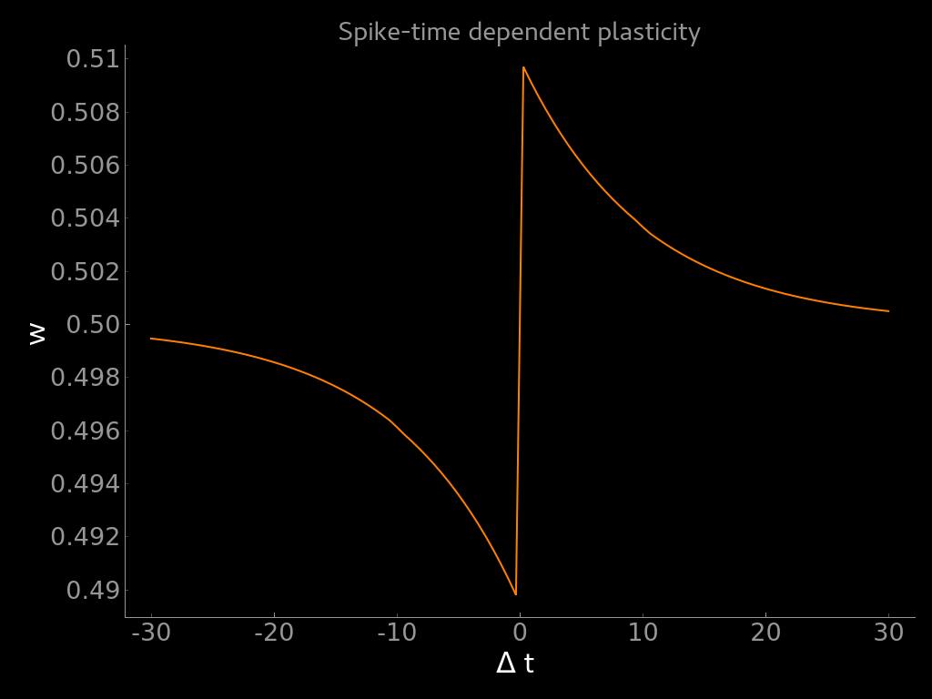
Visualization of the weight update as a function of the difference between post- and pre-synaptic spike times (dw = t_post - t_pre).
Add mismatch
Most spiking neural network models use homogeneous model parameters, such as synaptic time constants, spiking thresholds etc.
Biological neurons and synapses, however, show high diversity in their morphology and thus in their behaviour which is modelled using model parameters.
This diversity, i.e. heterogeneity, leads to highly variable responses which are usually not considered.
On the one hand, this heterogeneity might be actually relevant for computation and stability, thus should be encapsulated in spiking neural network models.
On the other hand neuromorphic mixed-signal analogue-digital sensory-processing systems are subject to so-called device mismatch due to imperfections in the manufacturing process.
To better assess if a given model is suited for an implementation on neuromorphic hardware and to advance our understanding of computation in heterogeneous population of neurons teili provides a Group level method to add device mismatch.
This example shows how to add device mismatch to a neural network with one input neuron connected to 1000 output neurons.
Once our population is created, we will add device mismatch to the selected parameters by specifying a dictionary with parameter names as keys and mismatch standard deviation as values.
The following tutorial can be found at ~/teiliApps/examples/mismatch_tutorial.py.
Here the selected parameters for the neuron and synapse models are specified in mismatch_neuron_param and mismatch_synap_param respectively.
import pyqtgraph as pg
import numpy as np
from brian2 import SpikeGeneratorGroup, SpikeMonitor, StateMonitor, second, ms, asarray, nA, prefs
from teili.core.groups import Neurons, Connections
from teili import TeiliNetwork
from teili.models.neuron_models import DPI as neuron_model
from teili.models.synapse_models import DPISyn as syn_model

from teili.tools.visualizer.DataModels.StateVariablesModel import StateVariablesModel
from teili.tools.visualizer.DataControllers.Rasterplot import Rasterplot
from teili.tools.visualizer.DataControllers.Lineplot import Lineplot
from teili.tools.visualizer.DataControllers.Histogram import Histogram
from teili.tools.visualizer.DataViewers import PlotSettings

prefs.codegen.target = "numpy"

Net = TeiliNetwork()

mismatch_neuron_param = {
    'Inoise' : 0,
    'Iconst' : 0,
    'kn' : 0,
    'kp' : 0,
    'Ut' : 0,
    'Io' : 0,
    'Cmem' : 0,
    'Iath' : 0,
    'Iagain' : 0,
    'Ianorm' : 0,
    'Ica' : 0,
    'Itauahp' : 0,
    'Ithahp' : 0,
    'Cahp' : 0,
    'Ishunt' : 0,
    'Ispkthr' : 0,
    'Ireset' : 0,
    'Ith' : 0,
    'Itau' : 0,
    'refP' : 0.2,
    }

mismatch_synap_param = {
    'Io_syn': 0,
    'kn_syn': 0,
    'kp_syn': 0,
    'Ut_syn': 0,
    'Csyn': 0,
    'I_tau': 0,
    'I_th': 0,
    'I_syn': 0,
    'w_plast': 0,
    'baseweight': 0.2
    }
This choice will add variability to the neuron refractory period (refP) and to the synaptic weight (baseweight), with a standard deviation of 20% of the current value for both parameters.
Let’s first create the input SpikeGeneratorGroup, the output layer and the synapses.
Notice that a constant input current has been set for the output neurons.
# Input layer
ts_input = asarray([1, 3, 4, 5, 6, 7, 8, 9]) * ms
ids_input = asarray([0, 0, 0, 0, 0, 0, 0, 0])
input_spikegen = SpikeGeneratorGroup(1, indices=ids_input,
                                     times=ts_input, name='gtestInp')

# Output layer
output_neurons = Neurons(1000, equation_builder=neuron_model(num_inputs=2),
                        name='output_neurons')
output_neurons.refP = 3 * ms
output_neurons.Iconst = 10 * nA

# Input Synapse
input_syn = Connections(input_spikegen, output_neurons, equation_builder=syn_model(),
                        name="inSyn", verbose=False)
input_syn.connect(True)
input_syn.weight = 5
Now we can add mismatch to the selected parameters.
First, we will store the current values of refP and baseweight to be able to compare them to those generated by adding mismatch (see mismatch distribution plot below).
Assuming that mismatch has not been added yet (e.g. if you have just created the neuron population), the values of the selected parameter will be the same for all the neurons in the population.
Here we will arbitrarily choose to store the first one.
neuron_param_mean = np.copy(getattr(output_neurons, 'refP'))[0]
neuron_param_unit = getattr(output_neurons, 'refP').unit
synapse_param_mean = np.copy(getattr(input_syn, 'baseweight'))[0]
synapse_param_unit = getattr(input_syn, 'baseweight').unit
Now we can add mismatch to neurons and synapses by using the method add_mismatch().
To be able to reproduce the same mismatch across multiple simulations and to use the same random distribution across bigger populations, we can also set the seed.
output_neurons.add_mismatch(std_dict=mismatch_neuron_param, seed=10)
input_syn.add_mismatch(std_dict=mismatch_synap_param, seed=11)
Once we run the simulation, we can visualize the effect of device mismatch on the EPSC and on the output membrane current Imem of five randomly selected neurons,
and the parameter distribution across neurons.
# Setting monitors:
spikemon_input = SpikeMonitor(input_spikegen, name='spikemon_input')
spikemon_output = SpikeMonitor(output_neurons, name='spikemon_output')
statemon_output = StateMonitor(output_neurons,
                                 variables=['Imem'],
                                 record=True,
                                 name='statemonNeuMid')
statemon_input_syn = StateMonitor(input_syn,
                                  variables='I_syn',
                                  record=True,
                                  name='statemon_input_syn')

Net.add(input_spikegen, output_neurons, input_syn,
                spikemon_input, spikemon_output,
                statemon_output, statemon_input_syn)

# Run simulation for 500 ms
duration = .500
Net.run(duration * second)
# define general settings
app = QtGui.QApplication.instance()
if app is None:
    app = QtGui.QApplication(sys.argv)
else:
    print('QApplication instance already exists: %s' % str(app))
    pg.setConfigOptions(antialias=True)
MyPlotSettings = PlotSettings(fontsize_title=12,
                              fontsize_legend=12,
                              fontsize_axis_labels=12,
                              marker_size=2)

# prepare data (part 1)
neuron_ids_to_plot = np.random.randint(1000, size=5)

distinguish_neurons_in_plot = True  # show values in different color per neuron otherwise the same color per subgroup

## plot EPSC (subfig3)
if distinguish_neurons_in_plot:
    # to get every neuron plotted with a different color to distinguish them
    DataModels_EPSC = []
    for neuron_id in neuron_ids_to_plot:
        MyData_EPSC = StateVariablesModel(state_variable_names=['EPSC'],
                                          state_variables=[statemon_input_syn.I_syn[neuron_id]],
                                          state_variables_times=[statemon_input_syn.t])
        DataModels_EPSC.append((MyData_EPSC, ('t_EPSC', 'EPSC')))
else:
    # to get all neurons plotted in the same color
    neuron_ids_to_plot = np.random.randint(1000, size=5)
    MyData_EPSC = StateVariablesModel(state_variable_names=['EPSC'],
                                 state_variables=[statemon_input_syn.I_syn[neuron_ids_to_plot].T],
                                 state_variables_times=[statemon_input_syn.t])
    DataModels_EPSC=[(MyData_EPSC, ('t_EPSC', 'EPSC'))]

## plot Imem (subfig4)
if distinguish_neurons_in_plot:
    # to get every neuron plotted with a different color to distinguish them
    DataModels_Imem = []
    for neuron_id in neuron_ids_to_plot:
        MyData_Imem = StateVariablesModel(state_variable_names=['Imem'],
                                          state_variables=[statemon_output.Imem[neuron_id].T],
                                          state_variables_times=[statemon_output.t])
        DataModels_Imem.append((MyData_Imem, ('t_Imem', 'Imem')))
else:
    # to get all neurons plotted in the same color
    neuron_ids_to_plot = np.random.randint(1000, size=5)
    MyData_Imem = StateVariablesModel(state_variable_names=['Imem'],
                                      state_variables=[statemon_output.Imem[neuron_ids_to_plot].T],
                                      state_variables_times=[statemon_output.t])
    DataModels_Imem=[(MyData_Imem, ('t_Imem', 'Imem'))]


# set up main window and subplots (part 1)
QtApp = QtGui.QApplication([])
mainfig = pg.GraphicsWindow(title='Simple SNN')
subfig1 = mainfig.addPlot(row=0, col=0)
subfig2 = mainfig.addPlot(row=1, col=0)
subfig3 = mainfig.addPlot(row=2, col=0)
subfig4 = mainfig.addPlot(row=3, col=0)

# add data to plots
Rasterplot(MyEventsModels=[spikemon_input],
                      MyPlotSettings=MyPlotSettings,
                      time_range=[0, duration],
                      title="Spike generator", xlabel="Time (ms)", ylabel="Neuron ID",
                      backend='pyqtgraph', mainfig=mainfig, subfig_rasterplot=subfig1, QtApp=QtApp,
                      show_immediately=False)
Rasterplot(MyEventsModels=[spikemon_output],
                     MyPlotSettings=MyPlotSettings,
                     time_range=[0, duration],
                     title="Output layer", xlabel="Time (ms)", ylabel="Neuron ID",
                     backend='pyqtgraph', mainfig=mainfig, subfig_rasterplot=subfig2, QtApp=QtApp,
                     show_immediately=False)
Lineplot(DataModel_to_x_and_y_attr=DataModels_EPSC,
                   MyPlotSettings=MyPlotSettings,
                   x_range=[0, duration],
                   title="EPSC", xlabel="Time (ms)", ylabel="EPSC (pA)",
                   backend='pyqtgraph', mainfig=mainfig, subfig=subfig3, QtApp=QtApp,
                   show_immediately=False)
Lineplot(DataModel_to_x_and_y_attr=DataModels_Imem,
                   MyPlotSettings=MyPlotSettings,
                   x_range=[0, duration],
                   title="I_mem", xlabel="Time (ms)", ylabel="Membrane current Imem (nA)",
                   backend='pyqtgraph', mainfig=mainfig, subfig=subfig4, QtApp=QtApp,
                   show_immediately=True)
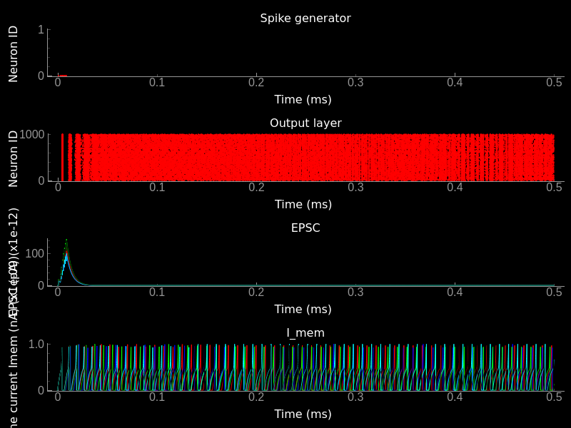
Effect of mismatch on neuron and synapse dynamics. Top) Input spike raster plot. Top/Middle) Output spike raster plot. Bottom/Middle) EPSC traces of different synapses. Note that the input spike time is the same but the temporal evolution, which is set by the synaptic paramters is different. Bottom) Traces of Imem of all neurons in the output population. Note that due to the heterogeneity the spike timing and the temporal dynamics differ for different neurons.
# Mismatch distribution
# prepare data (part 1)
input_syn_baseweights = np.asarray(getattr(input_syn, 'baseweight'))*10**12
MyData_baseweight = StateVariablesModel(state_variable_names=['baseweight'],
                                          state_variables=[input_syn_baseweights])  # to pA

refractory_periods = np.asarray(getattr(output_neurons, 'refP'))*10**3 # to ms
MyData_refP = StateVariablesModel(state_variable_names=['refP'],
                                  state_variables=[refractory_periods])

# set up main window and subplots (part 2)
mainfig = pg.GraphicsWindow(title='Mismatch distribution')
subfig1 = mainfig.addPlot(row=0, col=0)
subfig2 = mainfig.addPlot(row=1, col=0)

# add data to plots
Histogram(DataModel_to_attr=[(MyData_baseweight, 'baseweight')],
                    MyPlotSettings=MyPlotSettings,
                    title='baseweight', xlabel='(pA)', ylabel='count',
                    backend='pyqtgraph',
                    mainfig=mainfig, subfig=subfig1, QtApp=QtApp,
                    show_immediately=False)
y, x = np.histogram(input_syn_baseweights, bins="auto")
subfig1.plot(x=np.asarray([mean_synapse_param*10**12, mean_synapse_param*10**12]),
            y=np.asarray([0, 300]),
            pen=pg.mkPen((0, 255, 0), width=2))

Histogram(DataModel_to_attr=[(MyData_refP, 'refP')],
                    MyPlotSettings=MyPlotSettings,
                    title='refP', xlabel='(ms)', ylabel='count',
                    backend='pyqtgraph',
                    mainfig=mainfig, subfig=subfig2, QtApp=QtApp,
                    show_immediately=False)
subfig2.plot(x=np.asarray([neuron_param_mean*10**3, neuron_param_mean*10**3]),
             y=np.asarray([0, 450]),
        pen=pg.mkPen((0, 255, 0), width=2))

app.exec()
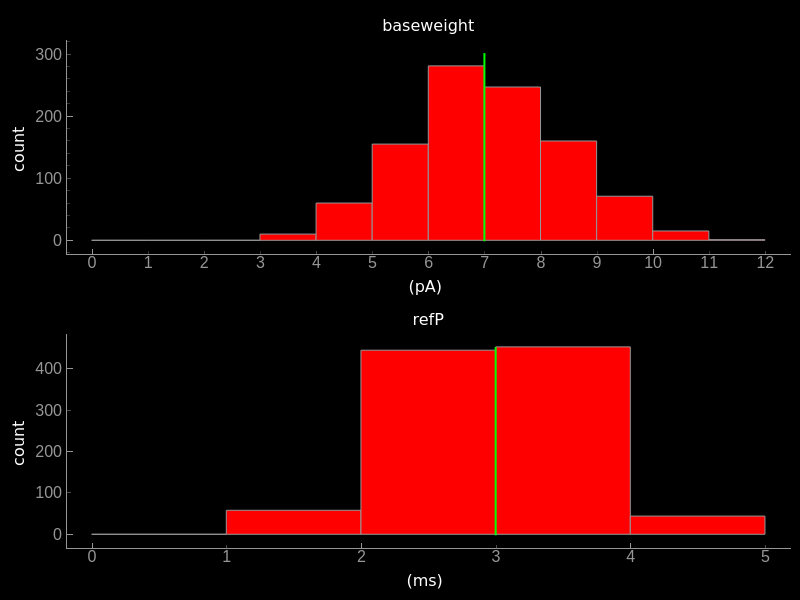
Effect of mismatch on paramters. Top) Histogram plot of baseweight. Bottom) Refractory period after mismatch has been applied. The mean value indicated by the yellow bar is the one specified in the parameters dictionary.
Re-building default models
To generate all pre-defined neuron and synapse models, which are stored by default in ~/teiliApps/equations/, please execute the following two scripts:
Note
During installation the static models are generated by default. You only need to re-generate them if you manually deleted or changed them and want the default static models.
from teili import neuron_models, synapse_models

synapse_models()
neuron_models()
Attention
If you develop your own custom models, make sure ro re-name them as all static models are re-compiled on install.
By default the models will be placed in teiliApps/equations/. If you want to place them at a different location follow the instructions below:
source activate <myenv>
python
from teili import neuron_models, synapse_models
neuron_models.main("/path/to/my/equations/")
synapse_models.main("/path/to/my/equations/")
Attention
You need to specify the absolute path. So use /home/<YOU>/your_custom_path/, rather than ~/your_custom_path/.
Note, that the following folder structure is generated in the specified location: /path/to/my/equations/teiliApps/equations/.
If you simply call the classes without a path the equations will be placed in ~/teiliApps/equations/.